library(dplyr)
flights <- nycflights13::flights7 Efficient data management
When working with data you must:
- Figure out what you want to do.
- Precisely describe what you want in the form of a computer program.
- Execute the code.
The dplyr package makes each of these steps as fast and easy as possible by:
- Elucidating the most common data manipulation operations, so that your options are helpfully constrained when thinking about how to tackle a problem.
- Providing simple functions that correspond to the most common data manipulation verbs, so that you can easily translate your thoughts into code.
- Using efficient data storage back ends, so that you spend as little time waiting for the computer as possible.
The nycflights13 package contains several data sets that can be used to help understand what causes delays. We will be using the flights data set which contains information about all flights that departed from NYC (e.g. EWR, JFK and LGA) in 2013.
7.1 Tibbles
The flights data set, and any data set created with dplyr, has a specific data type called a tibble. These are not as furry and prolific as their cousins the tribbles. tibbles behaves for all intents and purposes as a data.frame, just gets displayed differently. For example, the flights data set contains data on 19 characteristics (variables) from 336,776 flights. There’s no way I would want to print out a data set that large. But I’m gonna….
flights# A tibble: 336,776 × 19
year month day dep_time sched_dep_time dep_delay arr_time sched_arr_time
<int> <int> <int> <int> <int> <dbl> <int> <int>
1 2013 1 1 517 515 2 830 819
2 2013 1 1 533 529 4 850 830
3 2013 1 1 542 540 2 923 850
4 2013 1 1 544 545 -1 1004 1022
5 2013 1 1 554 600 -6 812 837
6 2013 1 1 554 558 -4 740 728
7 2013 1 1 555 600 -5 913 854
8 2013 1 1 557 600 -3 709 723
9 2013 1 1 557 600 -3 838 846
10 2013 1 1 558 600 -2 753 745
# ℹ 336,766 more rows
# ℹ 11 more variables: arr_delay <dbl>, carrier <chr>, flight <int>,
# tailnum <chr>, origin <chr>, dest <chr>, air_time <dbl>, distance <dbl>,
# hour <dbl>, minute <dbl>, time_hour <dttm>The output has been trimmed to something more reasonable for our viewing pleasure. This may not seem such a big deal because R Studio already provides some level of truncation for our viewing pleasure, but when you accidentally print out 400 pages of data set in your homework assignment, your instructor (and your wallet if you print it without looking) won’t be happy.
7.2 Basic verbs
The dplyr package contains many functions to perform data manipulation “actions”, also called verbs. We will look at the following verbs:
filter(): Returns a subset of the rowsselect(): Returns only the listed columnsrename(): Renames the variables listedmutate(): Adds columns from existing datarelocate(): Moves the order of the columnsarrange(): Sorts the rows by the value of a variablecase_when(): A useful expansion ofifelsesummarise(): Reduces each group to a single row by calculating aggregate measuresgroup_by(): Groups a data set on a factor variable, such that all functions performed are then done on each level of the factor
7.2.1 Filter
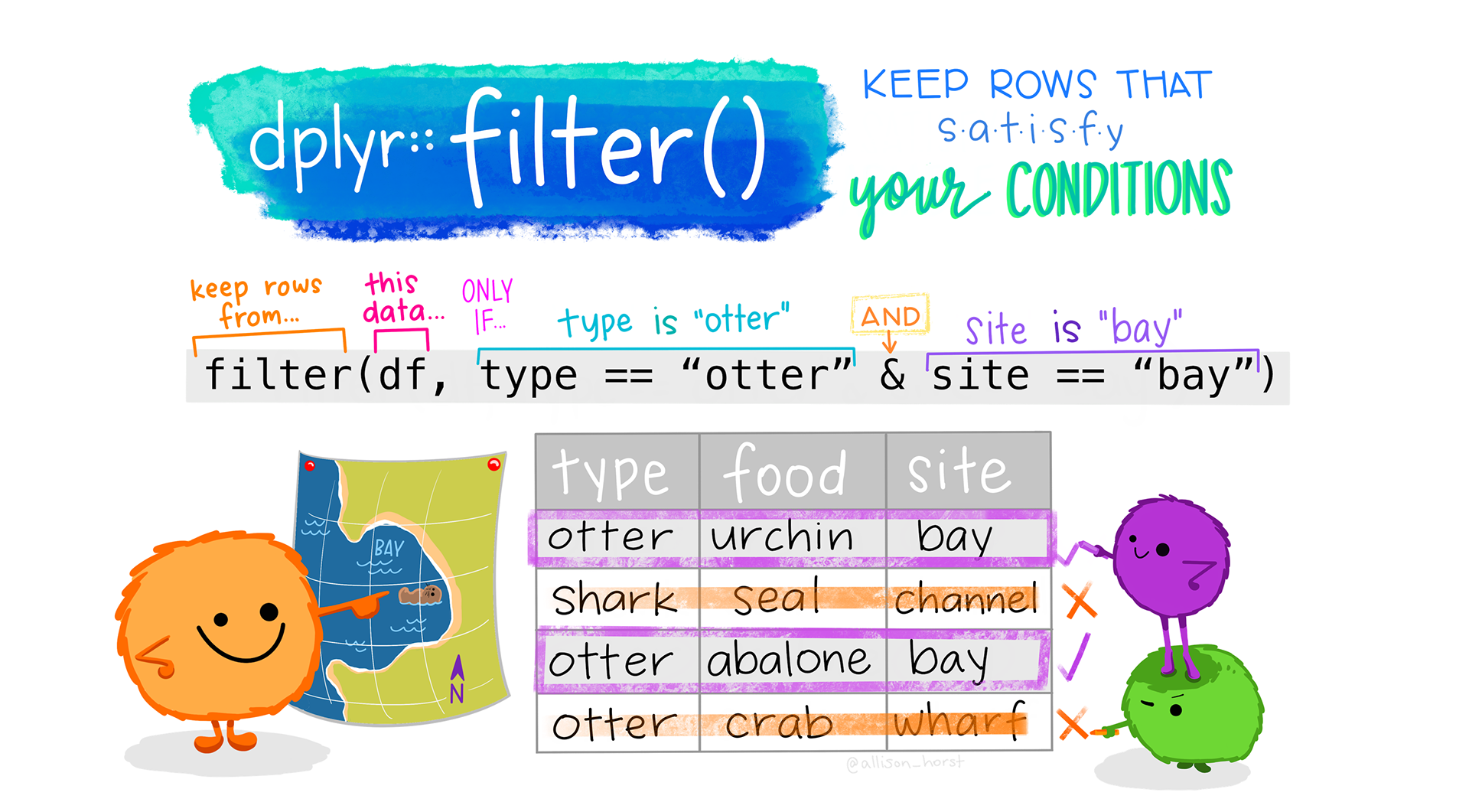
Learn more about dplyr::filter.
filter() allows you to select a subset of the rows of a data frame. The first argument is the name of the data frame, and the second and subsequent are filtering expressions evaluated in the context of that data frame. For example, we can select all flights on January 1st with
filter(flights, month == 1, day == 1)# A tibble: 842 × 19
year month day dep_time sched_dep_time dep_delay arr_time sched_arr_time
<int> <int> <int> <int> <int> <dbl> <int> <int>
1 2013 1 1 517 515 2 830 819
2 2013 1 1 533 529 4 850 830
3 2013 1 1 542 540 2 923 850
4 2013 1 1 544 545 -1 1004 1022
5 2013 1 1 554 600 -6 812 837
6 2013 1 1 554 558 -4 740 728
7 2013 1 1 555 600 -5 913 854
8 2013 1 1 557 600 -3 709 723
9 2013 1 1 557 600 -3 838 846
10 2013 1 1 558 600 -2 753 745
# ℹ 832 more rows
# ℹ 11 more variables: arr_delay <dbl>, carrier <chr>, flight <int>,
# tailnum <chr>, origin <chr>, dest <chr>, air_time <dbl>, distance <dbl>,
# hour <dbl>, minute <dbl>, time_hour <dttm>filter() works similarly to subset() except that you can give it any number of filtering conditions which are joined together with &. You can use other Boolean operators explicitly. Here we select flights in January or February.
filter(flights, month == 1 | month == 2)# A tibble: 51,955 × 19
year month day dep_time sched_dep_time dep_delay arr_time sched_arr_time
<int> <int> <int> <int> <int> <dbl> <int> <int>
1 2013 1 1 517 515 2 830 819
2 2013 1 1 533 529 4 850 830
3 2013 1 1 542 540 2 923 850
4 2013 1 1 544 545 -1 1004 1022
5 2013 1 1 554 600 -6 812 837
6 2013 1 1 554 558 -4 740 728
7 2013 1 1 555 600 -5 913 854
8 2013 1 1 557 600 -3 709 723
9 2013 1 1 557 600 -3 838 846
10 2013 1 1 558 600 -2 753 745
# ℹ 51,945 more rows
# ℹ 11 more variables: arr_delay <dbl>, carrier <chr>, flight <int>,
# tailnum <chr>, origin <chr>, dest <chr>, air_time <dbl>, distance <dbl>,
# hour <dbl>, minute <dbl>, time_hour <dttm>7.2.2 Select
Often you work with large data sets with many columns where only a few are actually of interest to you. select() allows you to rapidly zoom in on a useful subset using operations that usually only work on numeric variable positions.
select(flights, month, day, year)# A tibble: 336,776 × 3
month day year
<int> <int> <int>
1 1 1 2013
2 1 1 2013
3 1 1 2013
4 1 1 2013
5 1 1 2013
6 1 1 2013
7 1 1 2013
8 1 1 2013
9 1 1 2013
10 1 1 2013
# ℹ 336,766 more rowsYou can use a colon (:) to select all columns physically located between two variables.
select(flights, year:day)# A tibble: 336,776 × 3
year month day
<int> <int> <int>
1 2013 1 1
2 2013 1 1
3 2013 1 1
4 2013 1 1
5 2013 1 1
6 2013 1 1
7 2013 1 1
8 2013 1 1
9 2013 1 1
10 2013 1 1
# ℹ 336,766 more rowsTo exclude specific columns you use the minus sign (-)
select(flights, -carrier)# A tibble: 336,776 × 18
year month day dep_time sched_dep_time dep_delay arr_time sched_arr_time
<int> <int> <int> <int> <int> <dbl> <int> <int>
1 2013 1 1 517 515 2 830 819
2 2013 1 1 533 529 4 850 830
3 2013 1 1 542 540 2 923 850
4 2013 1 1 544 545 -1 1004 1022
5 2013 1 1 554 600 -6 812 837
6 2013 1 1 554 558 -4 740 728
7 2013 1 1 555 600 -5 913 854
8 2013 1 1 557 600 -3 709 723
9 2013 1 1 557 600 -3 838 846
10 2013 1 1 558 600 -2 753 745
# ℹ 336,766 more rows
# ℹ 10 more variables: arr_delay <dbl>, flight <int>, tailnum <chr>,
# origin <chr>, dest <chr>, air_time <dbl>, distance <dbl>, hour <dbl>,
# minute <dbl>, time_hour <dttm>This also works to exclude all columns EXCEPT the ones between two variables.
select(flights, -(year:day))# A tibble: 336,776 × 16
dep_time sched_dep_time dep_delay arr_time sched_arr_time arr_delay carrier
<int> <int> <dbl> <int> <int> <dbl> <chr>
1 517 515 2 830 819 11 UA
2 533 529 4 850 830 20 UA
3 542 540 2 923 850 33 AA
4 544 545 -1 1004 1022 -18 B6
5 554 600 -6 812 837 -25 DL
6 554 558 -4 740 728 12 UA
7 555 600 -5 913 854 19 B6
8 557 600 -3 709 723 -14 EV
9 557 600 -3 838 846 -8 B6
10 558 600 -2 753 745 8 AA
# ℹ 336,766 more rows
# ℹ 9 more variables: flight <int>, tailnum <chr>, origin <chr>, dest <chr>,
# air_time <dbl>, distance <dbl>, hour <dbl>, minute <dbl>, time_hour <dttm>7.2.3 Rename
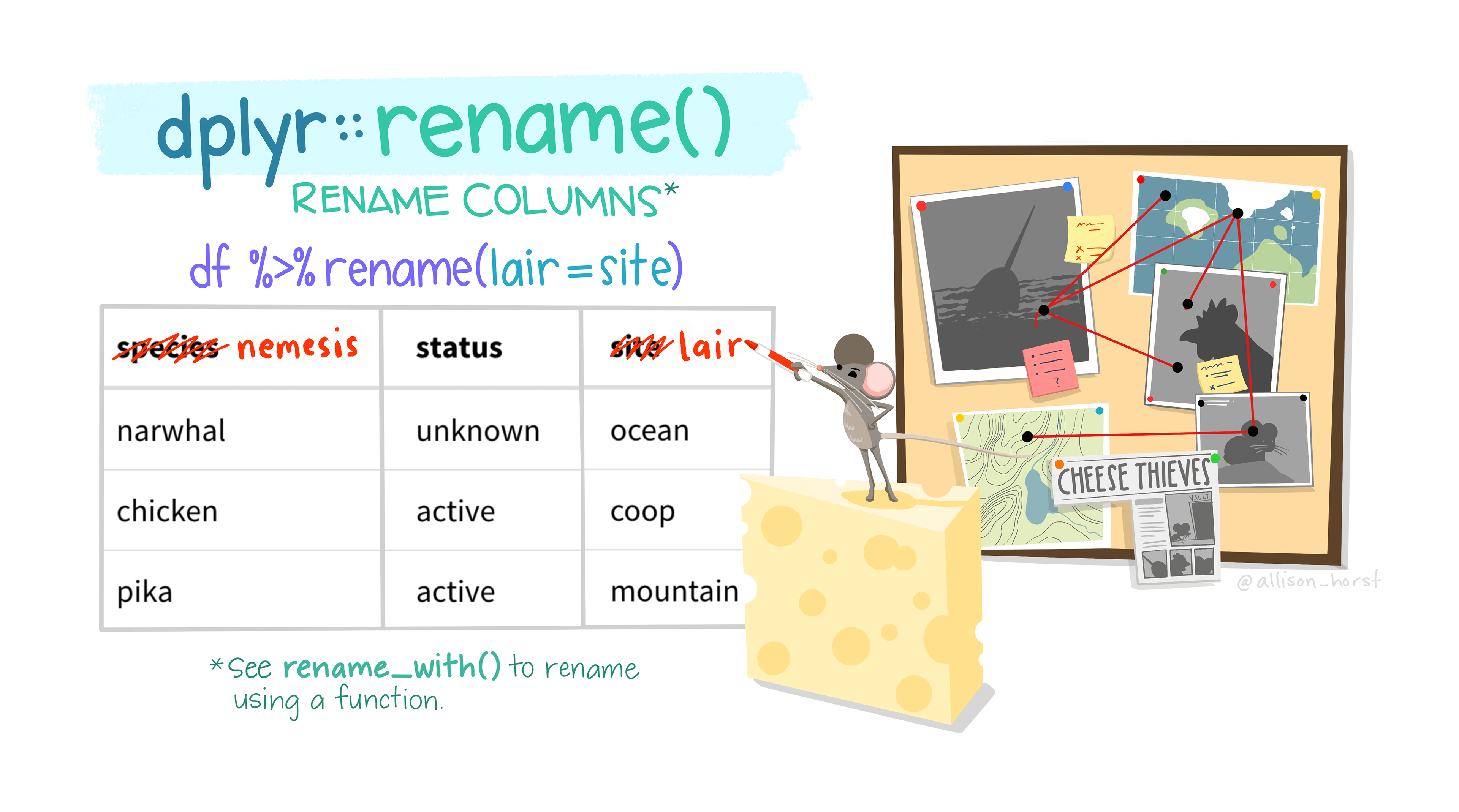
Learn more about dplyr::rename
Sometimes variables come to you in really obscure naming conventions. What the heck is SBA641? The rename() function converts an old name to a new name. The generic syntax is rename(new = old).
For the purpose of these lecture notes I am not making this change permanent. There is no assignment operator
<- used here, so this change is not going to persist into later code.So to rename dep_time to departure_time we would type
rename(flights, departure_time = dep_time)# A tibble: 336,776 × 19
year month day departure_time sched_dep_time dep_delay arr_time
<int> <int> <int> <int> <int> <dbl> <int>
1 2013 1 1 517 515 2 830
2 2013 1 1 533 529 4 850
3 2013 1 1 542 540 2 923
4 2013 1 1 544 545 -1 1004
5 2013 1 1 554 600 -6 812
6 2013 1 1 554 558 -4 740
7 2013 1 1 555 600 -5 913
8 2013 1 1 557 600 -3 709
9 2013 1 1 557 600 -3 838
10 2013 1 1 558 600 -2 753
# ℹ 336,766 more rows
# ℹ 12 more variables: sched_arr_time <int>, arr_delay <dbl>, carrier <chr>,
# flight <int>, tailnum <chr>, origin <chr>, dest <chr>, air_time <dbl>,
# distance <dbl>, hour <dbl>, minute <dbl>, time_hour <dttm>The variable name on the 3rd column now says departure_time instead of dep_time.
7.2.4 Mutate
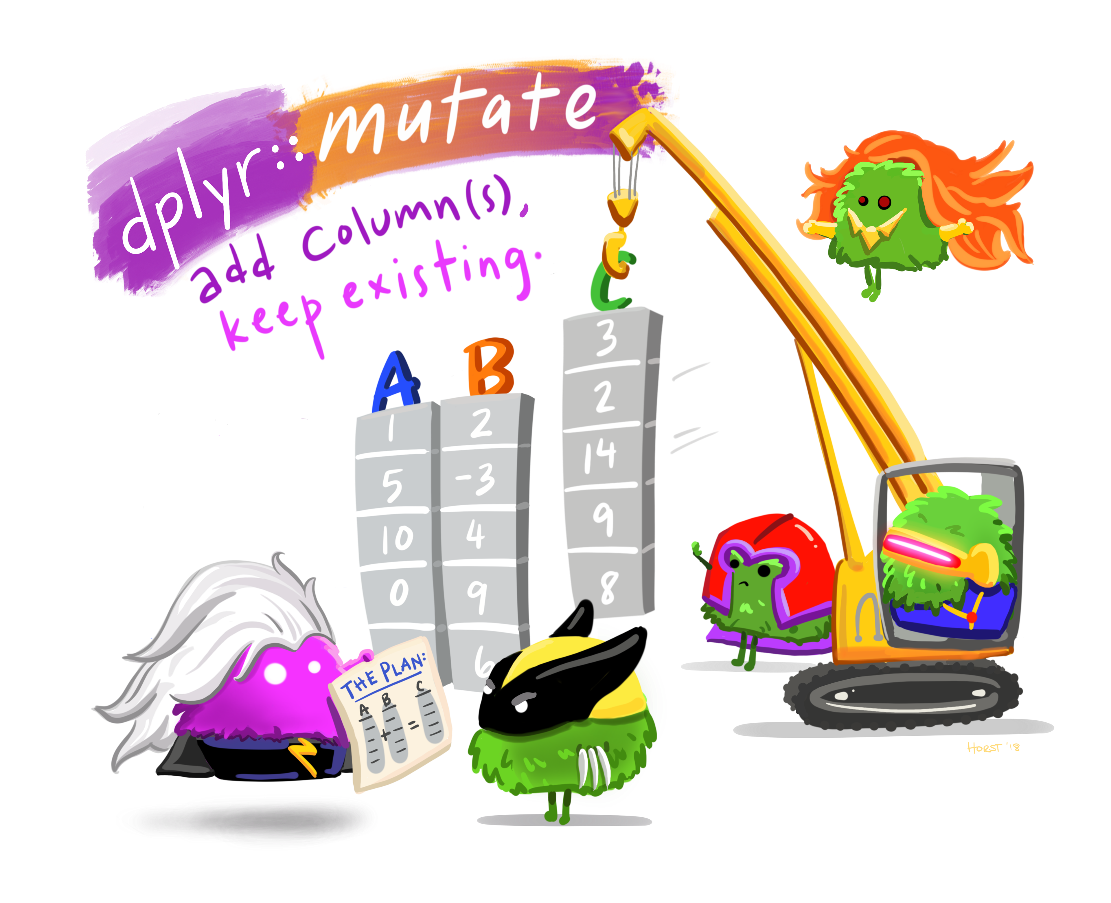
Learn more about dplyr::mutate
As well as selecting from the set of existing columns, it’s often useful to add new columns that are functions of existing columns. This is the job of mutate()!
Here we create two variables: gain (as arrival delay minus departure delay) and speed (as distance divided by time, converted to hours).
a <- mutate(flights, gain = arr_delay - dep_delay,
                speed = distance / air_time * 60)
select(a, gain, distance, air_time, speed)
# A tibble: 336,776 × 4
gain distance air_time speed
<dbl> <dbl> <dbl> <dbl>
1 9 1400 227 370.
2 16 1416 227 374.
3 31 1089 160 408.
4 -17 1576 183 517.
5 -19 762 116 394.
6 16 719 150 288.
7 24 1065 158 404.
8 -11 229 53 259.
9 -5 944 140 405.
10 10 733 138 319.
# ℹ 336,766 more rowsOne key advantage of mutate is that you can refer to the columns you just created. In one mutate call we can create the gain variable, and then use it to create gain_per_hour.
mutate(flights, gain = arr_delay - dep_delay,
                gain_per_hour = gain / (air_time / 60 ))
# A tibble: 336,776 × 21
year month day dep_time sched_dep_time dep_delay arr_time sched_arr_time
<int> <int> <int> <int> <int> <dbl> <int> <int>
1 2013 1 1 517 515 2 830 819
2 2013 1 1 533 529 4 850 830
3 2013 1 1 542 540 2 923 850
4 2013 1 1 544 545 -1 1004 1022
5 2013 1 1 554 600 -6 812 837
6 2013 1 1 554 558 -4 740 728
7 2013 1 1 555 600 -5 913 854
8 2013 1 1 557 600 -3 709 723
9 2013 1 1 557 600 -3 838 846
10 2013 1 1 558 600 -2 753 745
# ℹ 336,766 more rows
# ℹ 13 more variables: arr_delay <dbl>, carrier <chr>, flight <int>,
# tailnum <chr>, origin <chr>, dest <chr>, air_time <dbl>, distance <dbl>,
# hour <dbl>, minute <dbl>, time_hour <dttm>, gain <dbl>, gain_per_hour <dbl>7.2.5 Summarize
Next up is the verb summarise(), which is most often used to calculate summary statistics.
summarise(flights,
          ave_departure_delay = mean(dep_delay, na.rm = TRUE),
          n_flights_with_delay = sum(!is.na(dep_delay)>0),
          max_depart_delay = max(dep_delay, na.rm=TRUE)
)
# A tibble: 1 × 3
ave_departure_delay n_flights_with_delay max_depart_delay
<dbl> <int> <dbl>
1 12.6 328521 1301It may seem like a lot of code compared to base R functions such as mean(), sum() and max(), but we’ll see how this is used in combination with grouping in the next section to easily create grouped summary statistics.
7.2.6 Arrange
The arrange() function changes the order of the rows for the whole data set based on the value of the variable being sorted.
Lets use a smaller data set with fewer variables so it’s easier to visualize.
flights2 <- select(flights, distance, origin, dep_delay)7.2.6.1 Sort by one variable
Sort flights based on distance, from shortest to longest. This is Ascending order.
arrange(flights2, distance)# A tibble: 336,776 × 3
distance origin dep_delay
<dbl> <chr> <dbl>
1 17 EWR NA
2 80 EWR -2
3 80 EWR 40
4 80 EWR 134
5 80 EWR -1
6 80 EWR -5
7 80 EWR -4
8 80 EWR -5
9 80 EWR -3
10 80 EWR -3
# ℹ 336,766 more rowsTo reverse the sort order, use desc(). This is Descending order.
arrange(flights2, desc(distance))# A tibble: 336,776 × 3
distance origin dep_delay
<dbl> <chr> <dbl>
1 4983 JFK -3
2 4983 JFK 9
3 4983 JFK 14
4 4983 JFK 0
5 4983 JFK -2
6 4983 JFK 79
7 4983 JFK 102
8 4983 JFK 1
9 4983 JFK 1301
10 4983 JFK -1
# ℹ 336,766 more rows7.2.6.2 Sort by two variables
You can sort by more than one variable. Rows are ordered by the first variable, and ties are broken using the second variable.
Here we sort flights first by origin airport, then by departure delay within each airport.
arrange(flights2, origin, dep_delay)# A tibble: 336,776 × 3
distance origin dep_delay
<dbl> <chr> <dbl>
1 631 EWR -25
2 200 EWR -23
3 200 EWR -23
4 200 EWR -22
5 266 EWR -22
6 2402 EWR -21
7 200 EWR -21
8 200 EWR -21
9 937 EWR -20
10 1065 EWR -20
# ℹ 336,766 more rows
Avoid the base
sort function
There is a sort and order functions in base R, but they operate on a single vector only. They do not keep all rows in a data frame together when sorting rows, so avoid using it.
7.2.7 Relocate
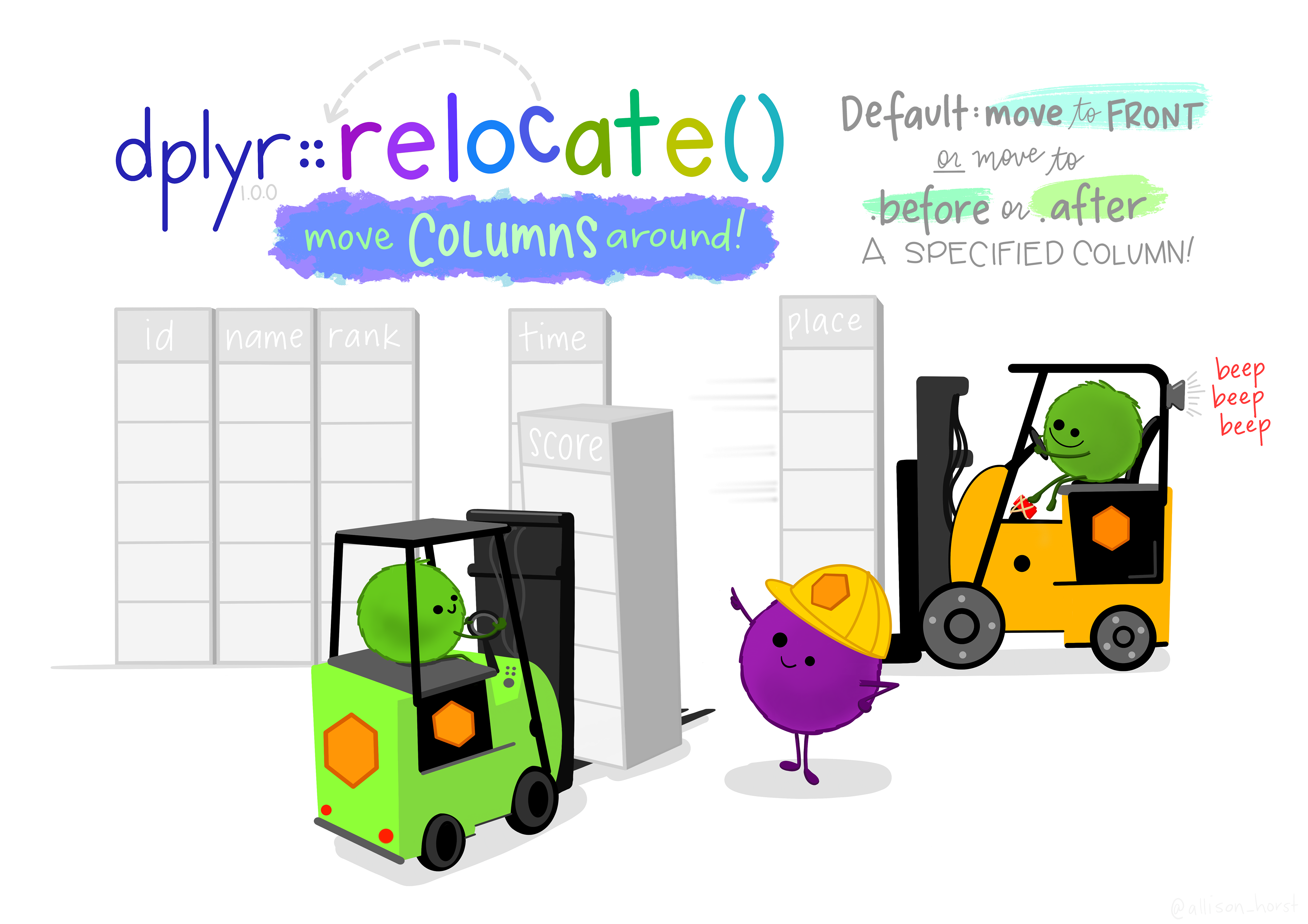
Learn more about dplyr::relocate
Use relocate() to change column positions, using the same syntax as select() to make it easy to move blocks of columns at once.
Current order of names for reference purposes.
names(flights) [1] "year" "month" "day" "dep_time"
[5] "sched_dep_time" "dep_delay" "arr_time" "sched_arr_time"
[9] "arr_delay" "carrier" "flight" "tailnum"
[13] "origin" "dest" "air_time" "distance"
[17] "hour" "minute" "time_hour" Bring origin to the front
flights <- flights %>%
  relocate(origin)
names(flights)
[1] "origin" "year" "month" "day"
[5] "dep_time" "sched_dep_time" "dep_delay" "arr_time"
[9] "sched_arr_time" "arr_delay" "carrier" "flight"
[13] "tailnum" "dest" "air_time" "distance"
[17] "hour" "minute" "time_hour" Move dest right after origin using the .after argument.
flights <- flights %>%
  relocate(dest, .after = origin)
names(flights)
[1] "origin" "dest" "year" "month"
[5] "day" "dep_time" "sched_dep_time" "dep_delay"
[9] "arr_time" "sched_arr_time" "arr_delay" "carrier"
[13] "flight" "tailnum" "air_time" "distance"
[17] "hour" "minute" "time_hour" Move multiple variables to the end
flights <- flights %>%
  relocate(c(carrier, flight, tailnum), .after = last_col())
names(flights)
[1] "origin" "dest" "year" "month"
[5] "day" "dep_time" "sched_dep_time" "dep_delay"
[9] "arr_time" "sched_arr_time" "arr_delay" "air_time"
[13] "distance" "hour" "minute" "time_hour"
[17] "carrier" "flight" "tailnum" 7.2.8 Case when
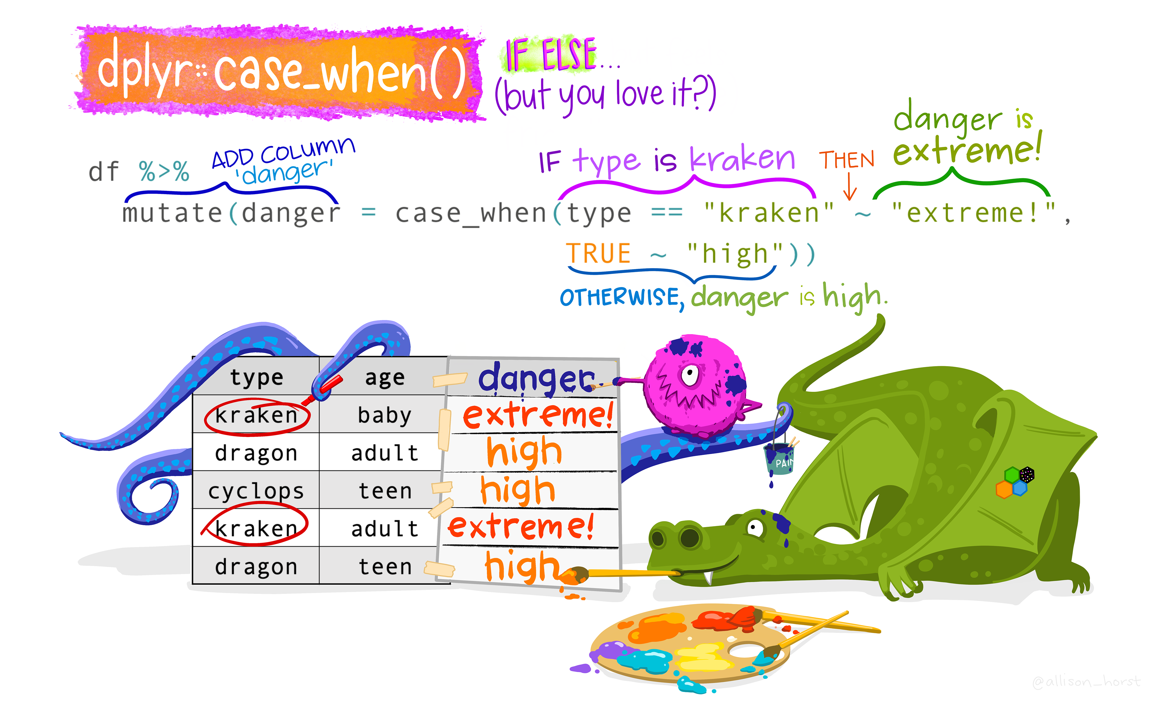
Learn more about case_when
This function allows you to vectorise multiple if_else() statements. Each case is evaluated sequentially and the first match for each element determines the corresponding value in the output vector. If no cases match, the .default is used as a final “else” statement.
The general syntax is logical statment ~ value. On the left hand side you specify a logical statement to identify a certain “case”, then a tilde ~, then on the right hand side you specify what you want the value of the new variable to be when this case is true.
1flights <- flights %>%
2  mutate(distance_cat = case_when(
3    distance <= 400 ~ "short",
4    distance > 400 & distance <= 1000 ~ "medium",
5    distance > 1000 ~ "long")
)- 1
-
Take the
flightsdata set, and then, - 2
-
Create a new variable called
distance_catwhere - 3
-
if the
distanceof the flight is less than or equal to 400 miles, set the value ofdistance_catto “short” - 4
-
if the
distanceis between 400 and 1000 miles, set the value ofdistance_catto “medium” - 5
-
if the
distanceis over 1000 miles, set the value ofdistance_catto “long”.
👉 Trust but verify
Create a grouped boxplot of distance against distance_cat to confirm that this recode worked.
Solution
ggpubr::ggboxplot(flights, y="distance", fill = "distance_cat")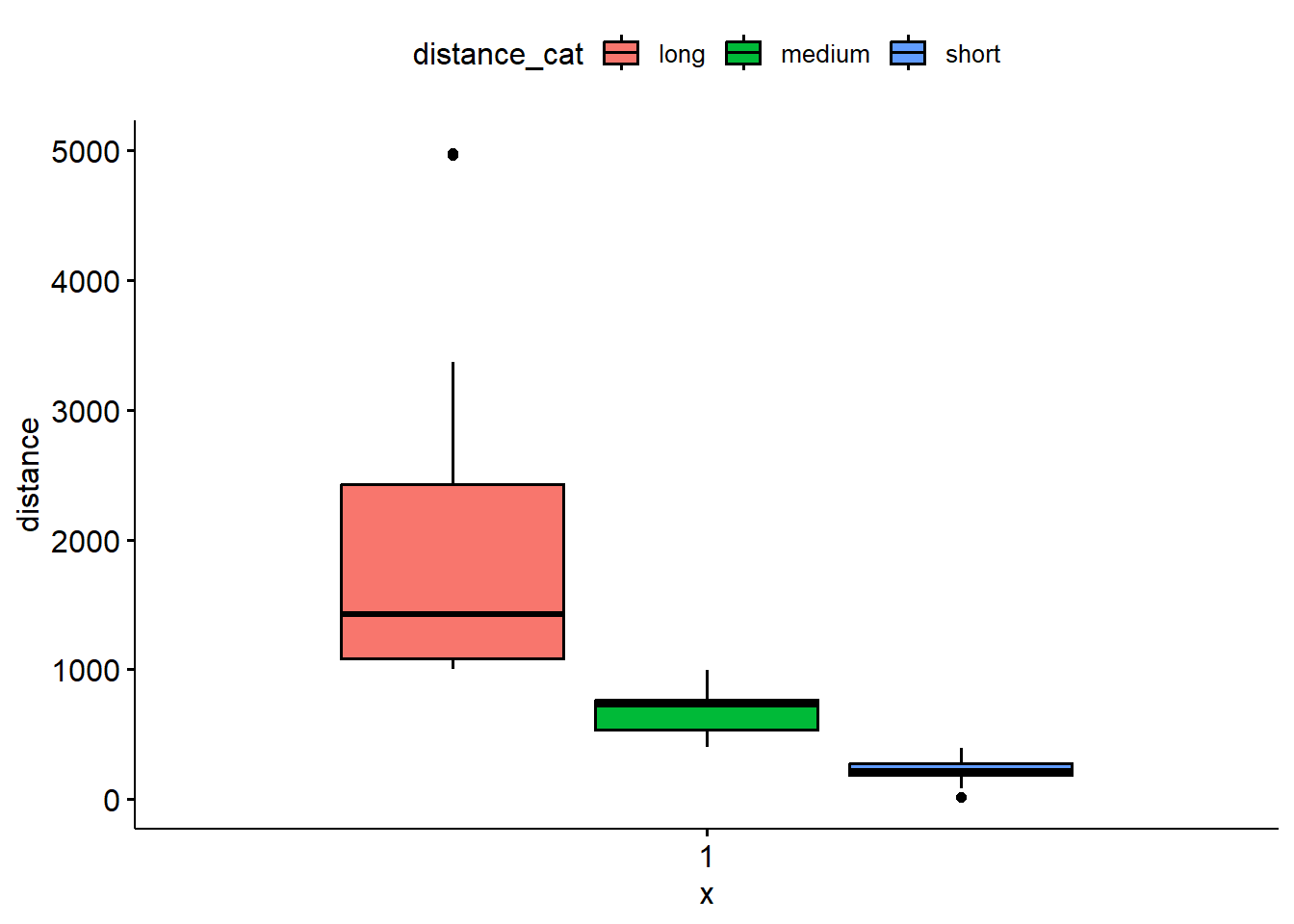
This case_when function can be used with complex logical statements involving multiple variables. Additionally, you don’t have to specify every single possible combination. If none of the statements specified evaluate as TRUE, the .default value will be used.
1flights <- flights %>%
2  mutate(delay_type = case_when(
             dep_delay > 0 & arr_delay > 0 ~ "two delays",
             dep_delay <= 0 & arr_delay <= 0 ~ "no delays",
3             TRUE ~ "one delay"
           )
  )
table(flights$delay_type, useNA="always")- 1
-
Take the
flightsdata set, and then, - 2
-
Create a new variable called
delay_typebased on whether or not there was a delay at both sides (departure and arrival), if there was no delays either departing or arriving - 3
-
If neither of these two statements are true, there is a delay at either the departure or arrival and so we set
delay_typeto “one delay”.
 no delays  one delay two delays       <NA>
    158900      85573      92303          0
7.3 Grouped Operations
The above verbs are useful, but they become really powerful when you combine them with the idea of “group by”, repeating the operation individually on groups of observations within the dataset. In dplyr, you use the group_by() function to describe how to break a dataset down into groups of rows. You can then use the resulting object in exactly the same functions as above; they’ll automatically work “by group” when the input is a grouped.
Let’s demonstrate how some of these functions work after grouping the flights data set by month. First we’ll create a new data set that is grouped by month.
by_month <- group_by(flights, month)The summarise() verb allows you to calculate summary statistics for each group. This is probably the most common function that is used in conjunction with group_by. For example, the average distance flown per month.
summarise(by_month, avg_distance = mean(distance, na.rm=TRUE))# A tibble: 12 × 2
month avg_distance
<int> <dbl>
1 1 1007.
2 2 1001.
3 3 1012.
4 4 1039.
5 5 1041.
6 6 1057.
7 7 1059.
8 8 1062.
9 9 1041.
10 10 1039.
11 11 1050.
12 12 1065.Or simply the total number of flights per month,
summarize(by_month, count=n())# A tibble: 12 × 2
month count
<int> <int>
1 1 27004
2 2 24951
3 3 28834
4 4 28330
5 5 28796
6 6 28243
7 7 29425
8 8 29327
9 9 27574
10 10 28889
11 11 27268
12 12 28135Or even more interestingly, the average departure delay, number of flights with delays, and the maximum length of delay at each of the three origin airports.
by_airport <- group_by(flights, origin)
summarise(by_airport,
          ave_departure_delay = mean(dep_delay, na.rm = TRUE),
          n_flights_with_delay = sum(!is.na(dep_delay)>0),
          max_depart_delay = max(dep_delay, na.rm=TRUE)
)
# A tibble: 3 × 4
origin ave_departure_delay n_flights_with_delay max_depart_delay
<chr> <dbl> <int> <dbl>
1 EWR 15.1 117596 1126
2 JFK 12.1 109416 1301
3 LGA 10.3 101509 911Seems like Laguardia (LGA) is the better airport for the least delays.
7.4 Chaining Operations
Same pipe, different symbol
We’ve seen chaining before using the base R pipe |>. The %>% symbol is also called a pipe, but is only accessible after you load the dplyr package. They function the same. We show both here because you will see both used out in the wild and need to know they are interchangeable.
Consider the following group of operations that take the data set flights, and produce a final data set (a4) that contains only the flights where the daily average delay is greater than a half hour.
a1 <- group_by(flights, year, month, day)
a2 <- select(a1, arr_delay, dep_delay)
a3 <- summarise(a2,
                arr = mean(arr_delay, na.rm = TRUE),
                dep = mean(dep_delay, na.rm = TRUE))
a4 <- filter(a3, arr > 30 | dep > 30)
head(a4)
# A tibble: 6 × 5
# Groups: year, month [3]
year month day arr dep
<int> <int> <int> <dbl> <dbl>
1 2013 1 16 34.2 24.6
2 2013 1 31 32.6 28.7
3 2013 2 11 36.3 39.1
4 2013 2 27 31.3 37.8
5 2013 3 8 85.9 83.5
6 2013 3 18 41.3 30.1It does the trick, but what if you don’t want to save all the intermediate results (a1 - a3)? Well these verbs are function, so they can be wrapped inside other functions to create a nesting type structure.
filter(
  summarise(
    select(
      group_by(flights, year, month, day),
      arr_delay, dep_delay
    ),
    arr = mean(arr_delay, na.rm = TRUE),
    dep = mean(dep_delay, na.rm = TRUE)
  ),
  arr > 30 | dep > 30
)
Woah, that is HARD to read! This is difficult to read because the order of the operations is from inside to out, and the arguments are a long way away from the function. To get around this problem, dplyr provides the %>% operator. x %>% f(y) turns into f(x, y) so you can use it to rewrite multiple operations so you can read from left-to-right, top-to-bottom:
1flights %>%
2  group_by(year, month, day) %>%
3  select(arr_delay, dep_delay) %>%
4  summarise(
    arr = mean(arr_delay, na.rm = TRUE),
    dep = mean(dep_delay, na.rm = TRUE)
  ) %>%
5 filter(arr > 30 | dep > 30)- 1
-
Take the
flightsdata set and then, - 2
-
groupit by date and then, - 3
-
selects the necessary variables, and then, - 4
- calculate the mean arrival and departure delays, and then,
- 5
-
filterto only keep rows with a daily average delay over half hour.
# A tibble: 49 × 5
# Groups:   year, month [11]
    year month   day   arr   dep
   <int> <int> <int> <dbl> <dbl>
 1  2013     1    16  34.2  24.6
 2  2013     1    31  32.6  28.7
 3  2013     2    11  36.3  39.1
 4  2013     2    27  31.3  37.8
 5  2013     3     8  85.9  83.5
 6  2013     3    18  41.3  30.1
 7  2013     4    10  38.4  33.0
 8  2013     4    12  36.0  34.8
 9  2013     4    18  36.0  34.9
10  2013     4    19  47.9  46.1
# ℹ 39 more rows
The same 4 steps that resulted in the a4 data set, but without all the intermediate data saved! This can be very important when dealing with Big Data. R stores all data in memory, so if your little computer only has 2G of RAM and you’re working with a data set that is 500M in size, your computers memory will be used up fast. a1 takes 500M, a2 another 500M, by now your computer is getting slow. Make another copy at a3 and it gets worse, a4 now likely won’t even be able to be created because you’ll be out of memory.