```{r}
#| eval: false
2+2
```2 Reproducibility with Quarto
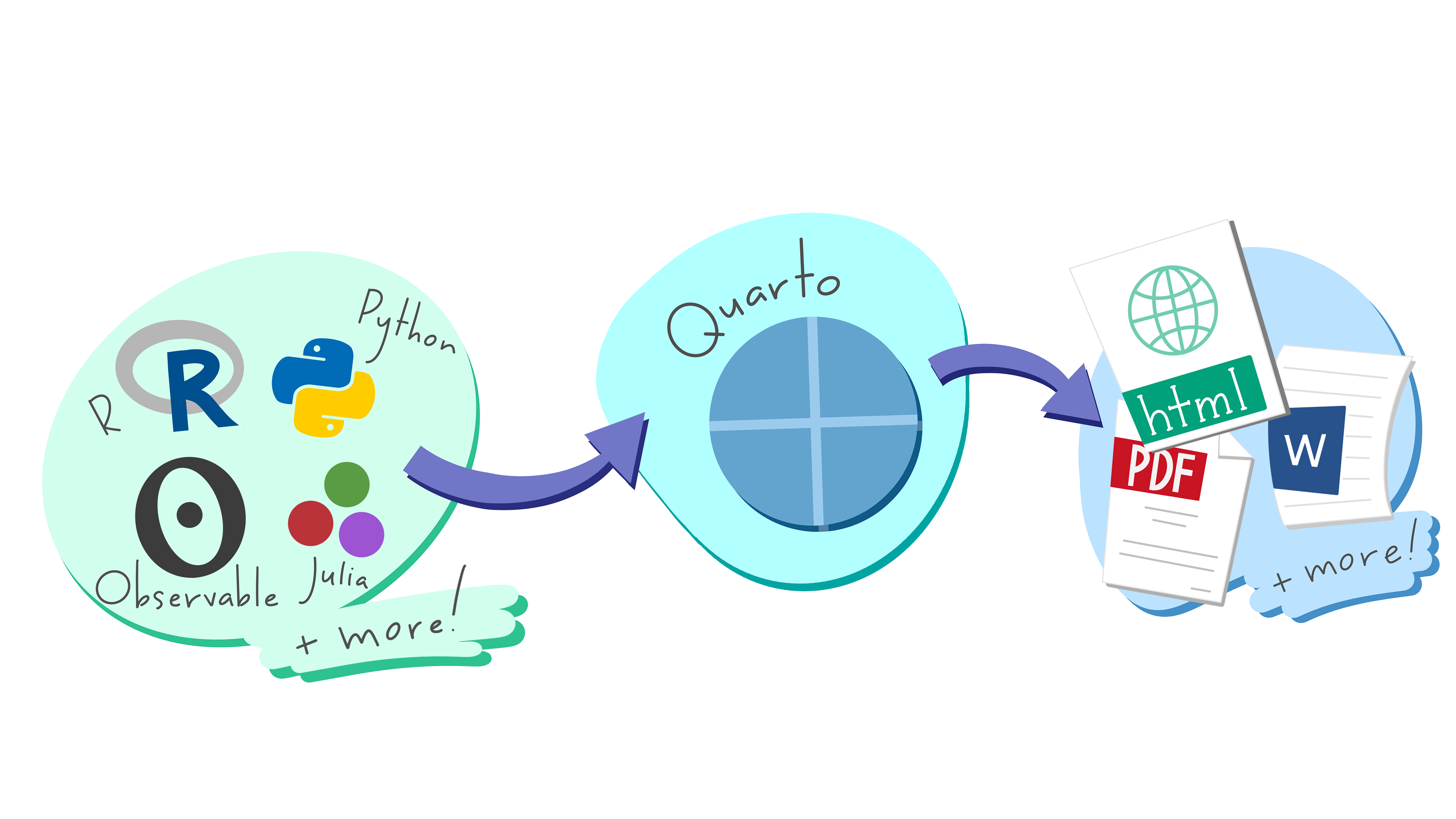
Quarto is a versatile publishing system that allows users to create high-quality documents, reports, websites (like this one!) and presentations using multiple programming languages like R, Python, and Julia. It combines the functionalities of various tools into a single platform, making it easier to produce reproducible and collaborative scientific content. If you have heard of R Markdown - Quarto is the “next generation” of R Markdown.
While Quarto is also it’s own standalone program, it comes “built-in” to R Studio so no additional installations needed!
2.1 Document structure
Quarto is an example of literate programming where the explanation of the program (or analysis) logic is presented in a natural language (such as English), with supporting pieces of code embedded in the document itself. Quarto combines normal text such as this sentence, code and the output from the code all in one file. It is similar to a scientific lab notebook where a scientist can write down their hypotheses, code to produce graphs and analysis results, and the discussion of those findings.
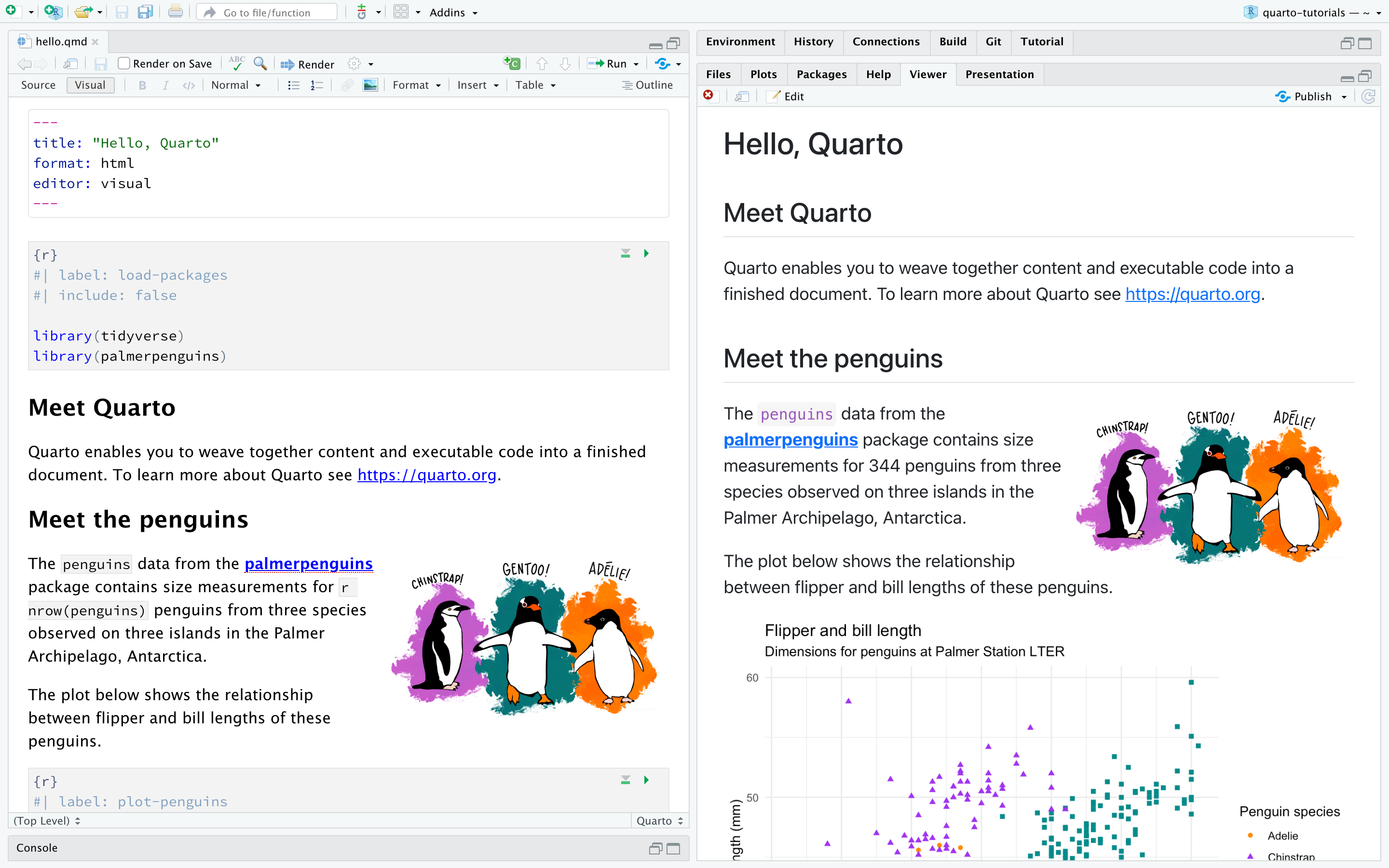
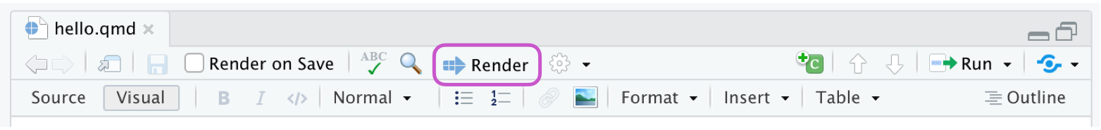
The ![]() Render button in the RStudio IDE compiles or renders the file and opens a preview of the output with a single click or keyboard shortcut SHIFT+COMMAND+K.
Render button in the RStudio IDE compiles or renders the file and opens a preview of the output with a single click or keyboard shortcut SHIFT+COMMAND+K.
2.2 Components of a Quarto file
Quarto files contains three types of content:
- A YAML header
- Code chunks
- Markdown text
2.2.1 YAML Header
An YAML header is demarcated by three dashes (—) on top and bottom. R is pretty finicky about these three dashes, so try not to disturb them.
When rendered, the title, "Hello, Quarto", will appear at the top of the rendered document with a larger font size than the rest of the document. The other two YAML fields denote that the output should be in html format and the document should open in the visual editor by default.
The basic syntax of YAML uses key-value pairs in the format key: value. Other YAML fields commonly found in headers of documents include metadata like author: and date:.
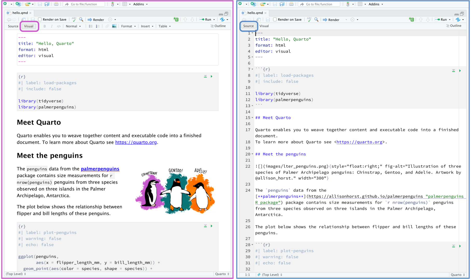
Visual vs Source mode RStudio’s Visual editor offers a WYSIWYM authoring experience for markdown formatting of text. Each view has it’s benefits and drawbacks, and which you choose to use is purely a matter of personal preference.
WYSIWYM: What You See Is What You Mean
2.2.2 Code Chunks
Code chunks start with three back ticks ``` and an {r} in braces. Chunks close (end) with another three back ticks.
a back tick is the key to the left of the 1 on your keyboardNote the background color of this section has changed to a different shade. This helps you identify you have closed your code chunk properly.
- You can insert code chunks by using the button in the top right of an RMD file (Insert -> R), or by typing CTRL+ALT+I.
- R code chunks can also have a YAML style header, prefixed by a “hash-pipe”
#|at the top of the code chunk. In this case I setevaltofalseto prevent the code inside this code chunk from being run when I render the whole document.
| is the first of three pipes we’ll see in this course
Only code goes in code chunks
That’s why they’re called code chunks. No normal text. All explanatory text goes outside code chunks in normal Markdown text.
In addition to rendering the complete document to view the results of code chunks, you can also run each code chunk interactively in the RStudio editor by clicking the play button icon in the top right corner of the code chunk, or keyboard shortcut CTRL + SHIFT + ENTER. RStudio executes the code and displays the results either inline within your file or in the Console, depending on your preference.
2.2.3 Markdown Text
Markdown is a popular markup language that allows you to add formatting elements to text. Markdown is useful because it is lightweight, flexible, and platform independent. [See more basic syntax of Markdown at https://quarto.org/docs/authoring/markdown-basics.html]{.aside}
| What you type | What you see |
|---|---|
**bold** |
bold |
_italics_ |
italics |
`code` |
code |
$2\beta - \frac{\mu}{n}$ |
\(2\beta - \frac{\mu}{n}\) |
| What you type | What you see |
|---|---|
|
|
|
|
Additionally, using # and ## symbols at the start of a line creates first (#) and second (##) level headers (larger font size, bold, numbered), such as Section 2.2 and line 15 in the hello.qmd file where it says ## Meet Quarto . Properly formatted headers are an important part of document organization and accessibility for screen reader navigation.
2.3 Create professional looking PDF reports.
To convert your work into a professional looking PDF, or to write math symbols in your homework, or you need a typesetting program called \(\LaTeX\) (pronounced “lay-tek” or “lah-tex”). It’s a super neat program, but also nearly 4Gb. Too big for our needs. That’s where the tinytex package came from. we’re going to use it to install a lightweight version of \(\LaTeX\). This will let us write math equations in Markdown/Quarto, and create nice PDF’s of your work.